
After reading this article, you will learn the Chi-Square Test and Probability theories and examples in detail
Chi-Square Test
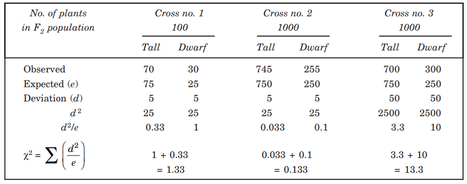
The size of the population is an important factor that must be considered when calculating chi-square or goodness of fit. Assume that in a single cross between tall and dwarf plants, out of the 100 plants that resulted in the F2 generation, 70 were tall and 30 were dwarf, rather than the 75 and 25 that would have been expected from a 3:1 ratio. The value is obviously off by 5, which indicates that there is a deviation.
Following the second cross, there were 745 tall plants and 255 dwarf ones among the F2 progeny of 1000 plants. This numerical variation was the same as that seen in the first cross. The third cross produced 1000 plants of the F2 generation in the same proportion as the first cross (70: 30 or 7: 3), which resulted in 700 tall plants and 300 dwarf plants.
The chi-square calculation, which is presented below, can be used to determine whether or not the observed variations in the results of the three crossings are statistically significant when compared to the 3:1 ratio. (Table.1).
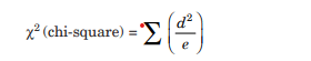
Where d represents a deviation from the expected ratio, e is the expected ratio, and Σ is the sum. The smaller the chi-square value, the more likely that deviation has occurred due to chance.
To determine if the disparities between expected and observed results are attributable to chance alone, we must first understand two more concepts: degree of freedom and level of significance.
Degrees of Freedom:
The number of degrees of freedom is equal to the number of classes whose values are necessary to represent the outcome from all classes. In experiments and genetic ratios, the concept of degrees of freedom is essential because the entire number of observed individuals must be considered a fixed or given quantity. This fixed amount consists of multiple variable classes.
There are just two classes in the experiment between tall and dwarf pea plants, tall and dwarf. Once the number of one class is identified, the number of the other can be determined. Therefore, there is one degree of freedom when scoring two classes.
When three classes are scored in an experiment, there are two degrees of freedom, and so on. The rule indicates that for the stated type of genetic studies, the number of classes is one less than the number of degrees of freedom.
Level of Significance:
In the described experiment, the actual ratio differs from the intended ratio. Now we must determine the significance of the disagreement in order to accept or reject the results.
Small disparities are not statistically significant, whereas large discrepancies are statistically significant and lead to the rejection of a result or hypothesis. Therefore, values are assigned to these two types of differences: the highest 5 percent of disparities are enormous, while the remaining 95 percent are tiny.
If the disagreement lies within the huge class, then it is substantial and the result may be disregarded. The frequency value of 5 percent that allows us to reject the result is known as the 5 percent level of significance. The importance level can be altered.
If 5 percent is too high, we can choose a lower significance level, such as 1 percent. In this instance, it is more difficult to reject a finding. In contrast, if we choose a high level of significance, such as 10%, it is simpler to reject a finding. Typically, the accepted level of significance is 5 percent, which falls between the two extremes.
After selecting the degrees of freedom and significance level in an experiment, chi-square is used to determine the real extent of the difference between expected and observed values.
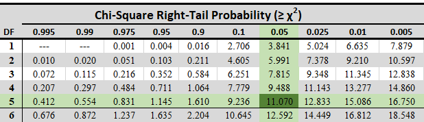
Statisticians have compiled tables that relate the number of degrees of freedom to the likelihood of locating particular chi-square value groupings (Table 2). Table IV from Fisher and Yates (1963) provides further information.
The findings of the experiment stated in Table 1 can now be examined. The first two crosses have chi-square values of 1.33 and 0.133. Both variances are acceptable because their values are less than Table 2’s chi-square value for one degree of freedom, which is 3.84.
The results of the first two crosses are therefore compatible with Mendel’s hypothesis, with the difference between expected and observed results traceable to random chance.
Probability:
Definition: Probability means likelihood. Probability theory is an area of mathematics concerned with the occurrence of random events. The value ranges between zero and one. Probability has been introduced in mathematics to predict the likelihood of occurrences occurring.
The definition of probability is the degree to which something is likely to occur. This is the fundamental theory of probability, which is also applied in the probability distribution, where you will discover the likelihood of random experiment outcomes. To determine the probability of a particular occurrence, we must first determine the total number of outcomes.
In the above-described trials, the F2 generation segregates in a specific proportion. The number of individuals in each ratio is the consequence of the random segregation of genes during gamete creation and the random combining of gametes to generate zygotes. Due to these occurrences’ random nature, accurate outcomes forecasts cannot be made.
This is especially true when the number of offspring is limited, as in animal breeding trials and even more so in human pedigree research. It is difficult to anticipate the occurrence of a particular phenotype or genotype. However, we can assert that a given genetic event is likely to occur.
In general, we can define the probability or chance that an event will occur as the fraction of times an event occurs throughout a large sample size. The probability is stated as y/x if there are x trials and the event occurs on average y times during those x trials. Between zero and one would be the probability.
The closer the probability is to zero, the less chance is there for the event to occur. When the probability is one, the event is sure to occur.Chi-Square Test and Probability
Probability Tree:
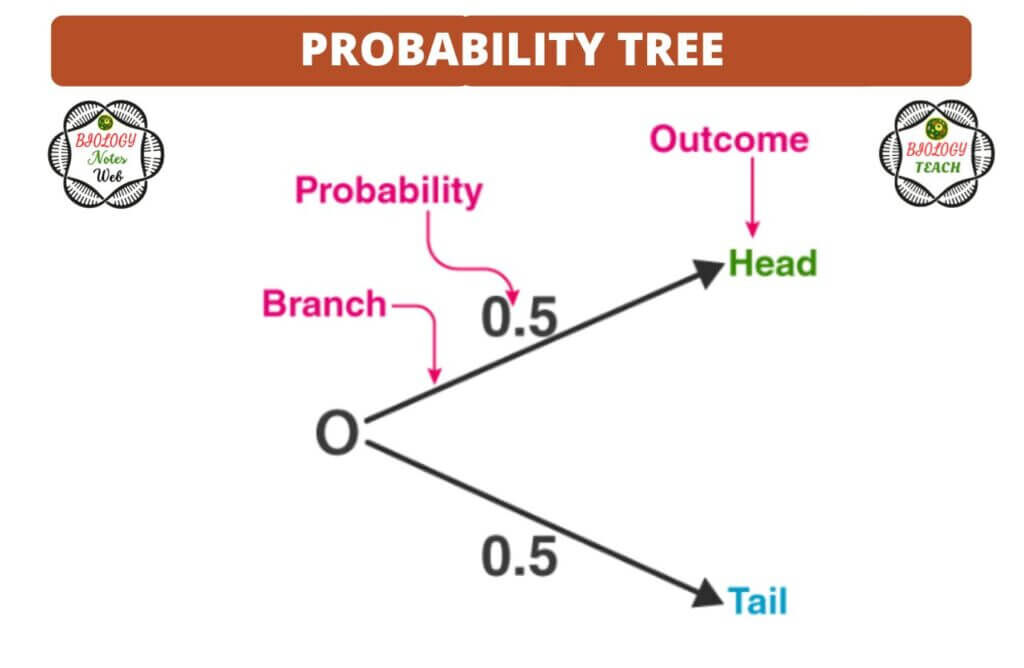
A tree diagram is a helpful tool for organizing and visualizing the various scenarios that could occur. There are two primary locations on the tree: the branches and the ends. On each branch is a printed indication of the probability of that branch’s conclusion, while the ends of the branches carry the ultimate result.
For the purpose of determining when to multiply and when to add, tree diagrams are utilized. An illustration of the coin in the form of a tree is shown below:
Types of Probability:
There are three major types of probabilities:
- Theoretical Probability
- Experimental Probability
- Axiomatic Probability
Theoretical Probability
It is based on the probability that something will occur. The theoretical probability highly depends on the logic behind probability. For instance, the theoretical probability of receiving a head while tossing a coin is 1/2.
Experimental Probability
It is derived from the observations of an experiment. The experimental probability can be estimated by dividing the total number of trials by the number of possible outcomes. For instance, if a coin is tossed ten times and heads are observed six times, the experimental probability for heads is 6/10, or 3/5.
Axiomatic Probability
In axiomatic probability, a set of principles or axioms that apply to all kinds are established. These axioms were established by Kolmogorov and are known as the three axioms of Kolmogorov. With the axiomatic approach to probability, the probabilities of events occurring or not occurring can be quantified. The lesson on axiomatic probability explains this topic in-depth with examples and Kolmogorov’s three rules (axioms).
Conditional Probability is the possibility that an event or result will occur based on the occurrence of a preceding event or result.
Rules of Probability:
When calculating probability, it is vital to remember that the inheritance of certain genes, such as those for pea plant height (tall or dwarf), flower color (red or white), and seed texture (round or wrinkled), are independent events. If we evaluate each gene separately, the probability that any given F2 plant will be tall is 3/4 and the probability that it would be short is 1/4.Chi-Square Test and Probability
Similarly, there is a 3/4 chance that an F2 plant will produce red flowers and a 1/4 chance that it will produce white flowers. What is the probability that an F2 plant is both tall and colored? Assuming that the inheritance of each gene is a separate event, the probability that a plant is both colorful and tall is equal to the product of their probabilities, or 3/4 3/4 = 9/16.
Therefore, nine out of sixteen F2 plants will be colorful and tall. When the chance of one event is independent of the probability of another event, and the occurrence of one event does not influence the occurrence of the other, the probability that both events will occur simultaneously is the product of their individual probabilities.
The Addition Rule states that the probability that one of several mutually exclusive events will occur is equal to the sum of the probabilities of the individual events. This law applies when distinct sorts of occurrences cannot occur simultaneously. If one occurs, the other cannot occur. When a coin is tossed, there are two possible outcomes: either heads or tails.
If the probability of heads is 1/2 and the probability of tails is 1/2, then the probability of either heads or tails is 1/2 + 1/2 = 1.
Probability and Human Genetics:
In humans with some recessive genetic traits, such as phenylketonuria (PKU), albinism, and others, the birth of an affected child implies that both parents are heterozygous carriers for that trait. Because the gene is recessive, the parents are healthy and normal. Such parents may wish to know the probability that their future children would exhibit the genetic flaw.
Since the characteristic is recessive, they could anticipate 1 afflicted child for every 3 normal offspring. Due to the restricted size of human families, however, this ratio can be deceiving. We can only state that the risk or probability of having a child with the condition is one-fourth at every birth. In addition, even after the delivery of one affected kid, the probability of having another affected child is the same (1/4) in all subsequent pregnancies.
At each birth, a normal child has a probability of 3/4. The rules of probability can be used to forecast the ratio of male to female births in a family. Since a human male generates an equal number of X and Y sperm, the probability of having a boy or a girl at any given birth is 50/50. From the chance of each conception, the probability of successive births can be calculated.
For instance, what is the probability that a family’s first two children will be boys? To determine this, we must double the probability of each conception, or 1/2 1/2 = 1/4. Now examine a different question.
What is the probability that the third child in a household with two male children will also be male? Remembering that the sex of any child is independent of the sex of the other children, the probability that the third child will be male is half.
Binomial Expansions of Probability:
There are countless incidents in genetics in which we would like to know the probability that a particular event combination would occur. For instance, it may be necessary to calculate the probability that two kids of Aa and aa parents will have a specific genetic composition, namely 2 Aa, 2 aa, or 1 Aa and the other aa.
The occurrence of a given genotype in a single offspring is an independent event, as the genotypes of any other offspring do not influence it. Therefore, the probability that this pairing would produce two Aa offspring is equal to the product of their probabilities. Chi-Square Test and Probability
Aa = 1/2 × 1/2 = 1/4 or 25%
Thus the probabilities for each sequence of two offspring”s are as follows:
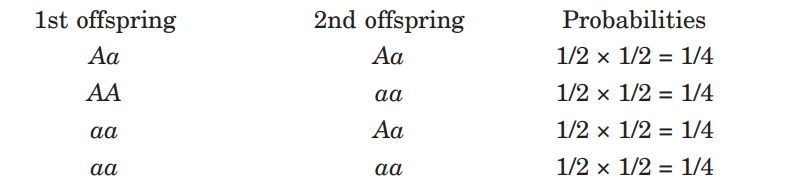
As a result, the probability that both of the kids are aa is 1/4, the probability that one of the offspring is Aa and the other is aa is 2/4, and the probability that both are aa is 1/4. To put it another way, the ratio of one to two to one describes the pattern of this distribution. This also shows the coefficients that are obtained by raising two different values of the binomial to the power of 2:
(p + q) 2 = 1p2 + 2pq + 1q2
or if we substitute Aa for p and aa for q
[(Aa) + (aa)]2 = 1(Aa) (Aa) + 2(Aa) (aa) + 1(aa) (aa)
It is important to remember that the chance of a complimentary event, such as the probability that both children will not be aa, is equal to 1 minus the probability of the specific event, which is written as 1 minus 1/4, which equals 3/4.
The frequencies of each genotype combination will be found to match with raising a binomial to the third power if the probabilities for the various combinations of genotypes that are possible among three children of the mating Aa aa are computed.
The probability that 3 offspring are Aa = 1/8
The probability that two are Aa and one aa = 3/8
The probability that two are aa and one Aa = 3/8
The probability that 3 offspring are aa = 1/8
or (p + q)3 = 1p3 + 3p2q + 3pq2 + 1q3
or [(Aa) + (aa)]3 = 1(Aa) (Aa) (Aa) + 3(Aa) (Aa) (aa) + 3(Aa) (aa) (aa) + 1(aa) (aa) (aa)
Therefore, the probability for each particular combination of children may be calculated by comparing the binomial coefficient for that combination to the total number of potential combinations. This will give the probability for that particular combination.
In general, we can say that when p is the probability that a particular event will occur and q or 1 – p is the probability of an alternative form of that event so that p + q = 1, then the binomial distribution describes the probability for each combination in which a succession of such events may occur. For example, if p is the probability that a particular event will occur, then q is the probability of an alternative form of that event.
Multinomial Distribution:
Only two different courses of action could be taken for each event in the instances that were just presented. There is the possibility that three distinct sorts of offspring could result from a genetic cross or mating. For example, an Aa Aa cross will result in the birth of AA, Aa, and aa offspring in the proportions of 1:2:1, which results in the following probabilities: 1/4 for AA, 1/2 for Aa, and 1/4 for aa.
When this occurs, a new term must be added to the binomial to properly express the third class of offspring. We have a trinomial distribution with the parameters p, q, and r, where p, q, and r, respectively reflect the probability of AA, Aa, and aa. For determining probabilities of trinomial combinations, we use the formula
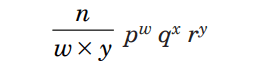
where w, x, and y represent the number of offspring of each of the three distinct types, and p, q, and r represent the corresponding probabilities of each of those offspring types occurring.
References:
- Chen, Yikai, et al. “Differences in Factors Affecting Various Crash Types with High Numbers of Fatalities and Injuries in China.” PLoS One, vol. 11, no. 7, Public Library of Science, July 2016, p. e0158559.
- “Peru : Free Line 113 Health Will Attend in Long Holiday.” MENA Report, Albawaba (London) Ltd., Nov. 2019.
- https://www.biologydiscussion.com
- https://books.google.com/books?id=FWbLBQAAQBAJ&printsec=frontcover&dq=biological+statics+book&hl=en&newbks=1&newbks_redir=1&sa=X&ved=2ahUKEwji6LnqjuL4AhVYIDQIHY2XBRUQ6AF6BAgHEAI